Exploring numerical data

based on IMS Ch 5: Exploring numerical data

Outline

• types of numerical data

• why visualize data

  • how to visualize two numerical variables
    • scatterplot
  • how to visualize one numerical variable
    • dot plot, histogram, density, box plot

What are the different types of numerical data?

• integer
  • examples
• double
  • examples

Why visualize data

• spot patterns and trends
• communicate data to others
• visual representation much more effective than table
• identify outliers
• explore data

Steps in data analysis

Load the packages

library(tidyverse)
library(openintro)
library(scales)
theme_set(theme_minimal()) #set theme of all plots to minimal

Dataset

• loan50 is part of the openintro packange

• automatically loaded when you call the library command

loan50

Glimpse the data

glimpse(loan50)

Rows: 50
Columns: 18
$ state                   <fct> NJ, CA, SC, CA, OH, IN, NY, MO, FL, FL, MD, HI…
$ emp_length              <dbl> 3, 10, NA, 0, 4, 6, 2, 10, 6, 3, 8, 10, 10, 2,…
$ term                    <dbl> 60, 36, 36, 36, 60, 36, 36, 36, 60, 60, 36, 36…
$ homeownership           <fct> rent, rent, mortgage, rent, mortgage, mortgage…
$ annual_income           <dbl> 59000, 60000, 75000, 75000, 254000, 67000, 288…
$ verified_income         <fct> Not Verified, Not Verified, Verified, Not Veri…
$ debt_to_income          <dbl> 0.55752542, 1.30568333, 1.05628000, 0.57434667…
$ total_credit_limit      <int> 95131, 51929, 301373, 59890, 422619, 349825, 1…
$ total_credit_utilized   <int> 32894, 78341, 79221, 43076, 60490, 72162, 2872…
$ num_cc_carrying_balance <int> 8, 2, 14, 10, 2, 4, 1, 3, 10, 4, 3, 4, 3, 2, 3…
$ loan_purpose            <fct> debt_consolidation, credit_card, debt_consolid…
$ loan_amount             <int> 22000, 6000, 25000, 6000, 25000, 6400, 3000, 1…
$ grade                   <fct> B, B, E, B, B, B, D, A, A, C, D, A, A, A, A, E…
$ interest_rate           <dbl> 10.90, 9.92, 26.30, 9.92, 9.43, 9.92, 17.09, 6…
$ public_record_bankrupt  <int> 0, 1, 0, 0, 0, 0, 0, 0, 0, 1, 0, 0, 0, 0, 0, 0…
$ loan_status             <fct> Current, Current, Current, Current, Current, C…
$ has_second_income       <lgl> FALSE, FALSE, FALSE, FALSE, FALSE, FALSE, FALS…
$ total_income            <dbl> 59000, 60000, 75000, 75000, 254000, 67000, 288…

Scatterplots

• show associations between variables

Scatterplots

• data = loan50

• x-axis = total_income

• y-axis = loan_amount

• geom_point: create scatterplot

  • ?geom_point() aesthetic options

ggplot(loan50, aes(x = total_income, y = loan_amount)) +
  geom_point()

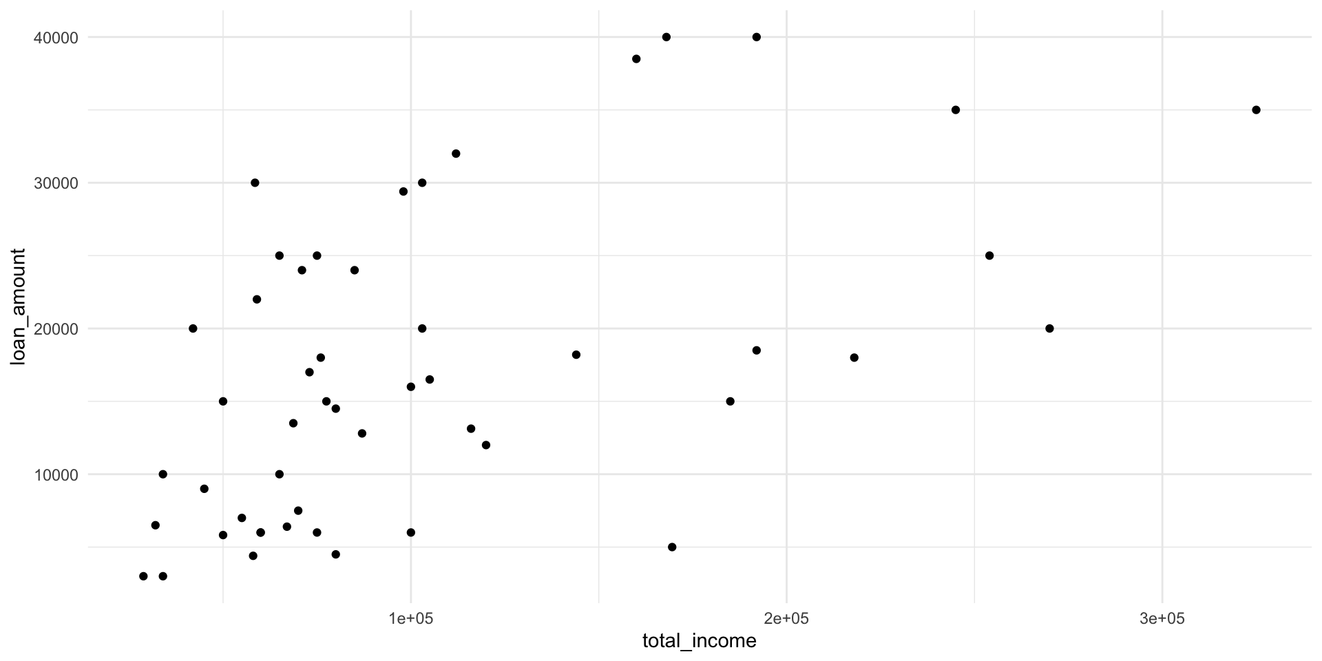
Scatterplot with formatting

ggplot(loan50, aes(x = total_income, y = loan_amount)) +
  geom_point(size = 3, color = "blue") +
  scale_x_continuous(labels = label_dollar(scale = 0.001, suffix = "K")) +
  scale_y_continuous(labels = label_dollar(scale = 0.001, suffix = "K")) +
  labs(x = "Total income", y = "Loan amount", title = "Scatterplot of loan amount and total income")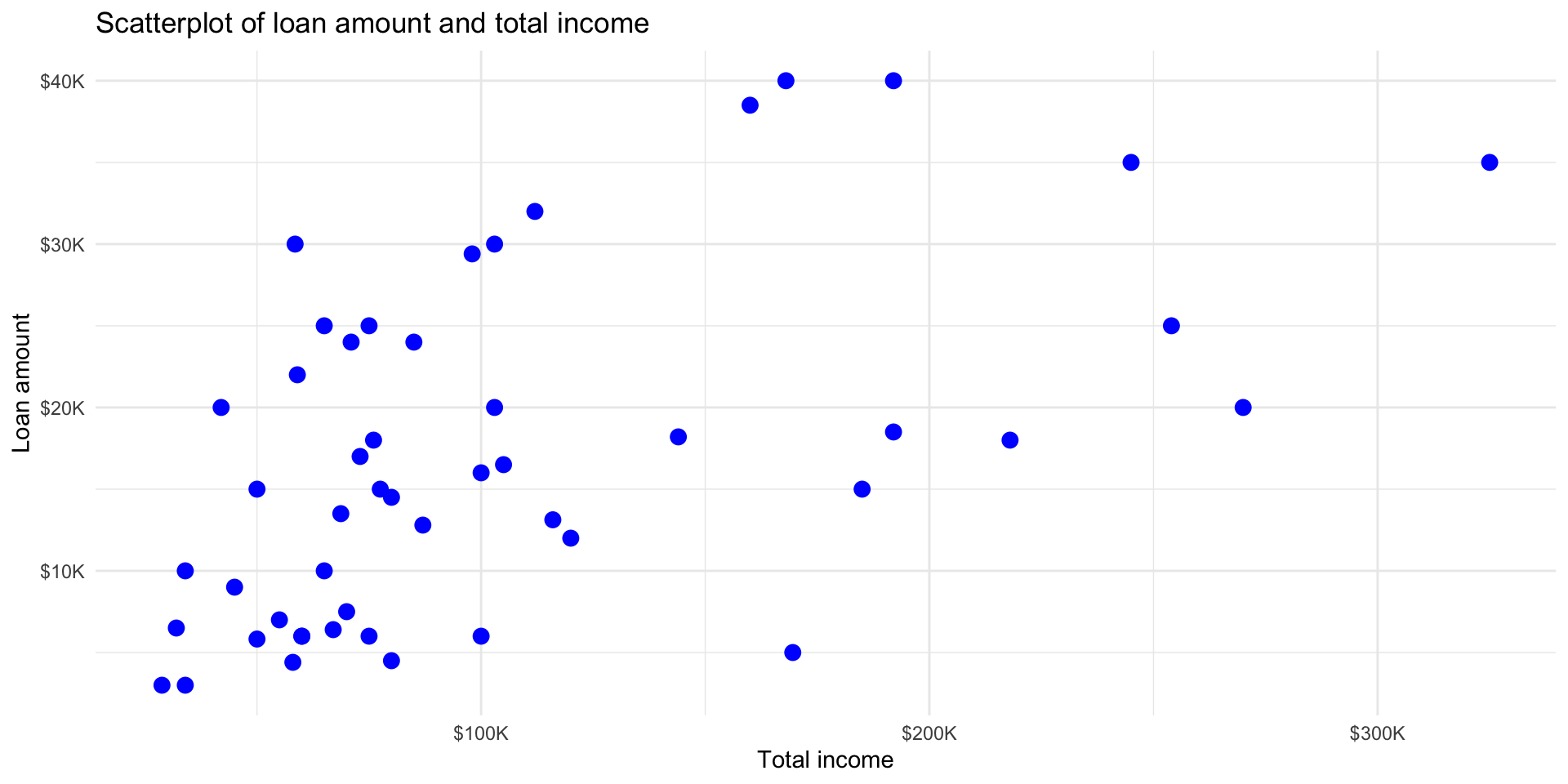

• What do you see?

Your turn - scatterplot

• Create a scatterplot of loan_amount on the x-axis and interest_rate on the y-axis

• Label the x axis in dollars

• Label the y axis in percent (hint: use label_percent with scale = 1)

• Add a title, label the x and y axes

Dot plots

• Plot distribution of one numerical variable
• Each dot represents an observation
• Dots are stacked

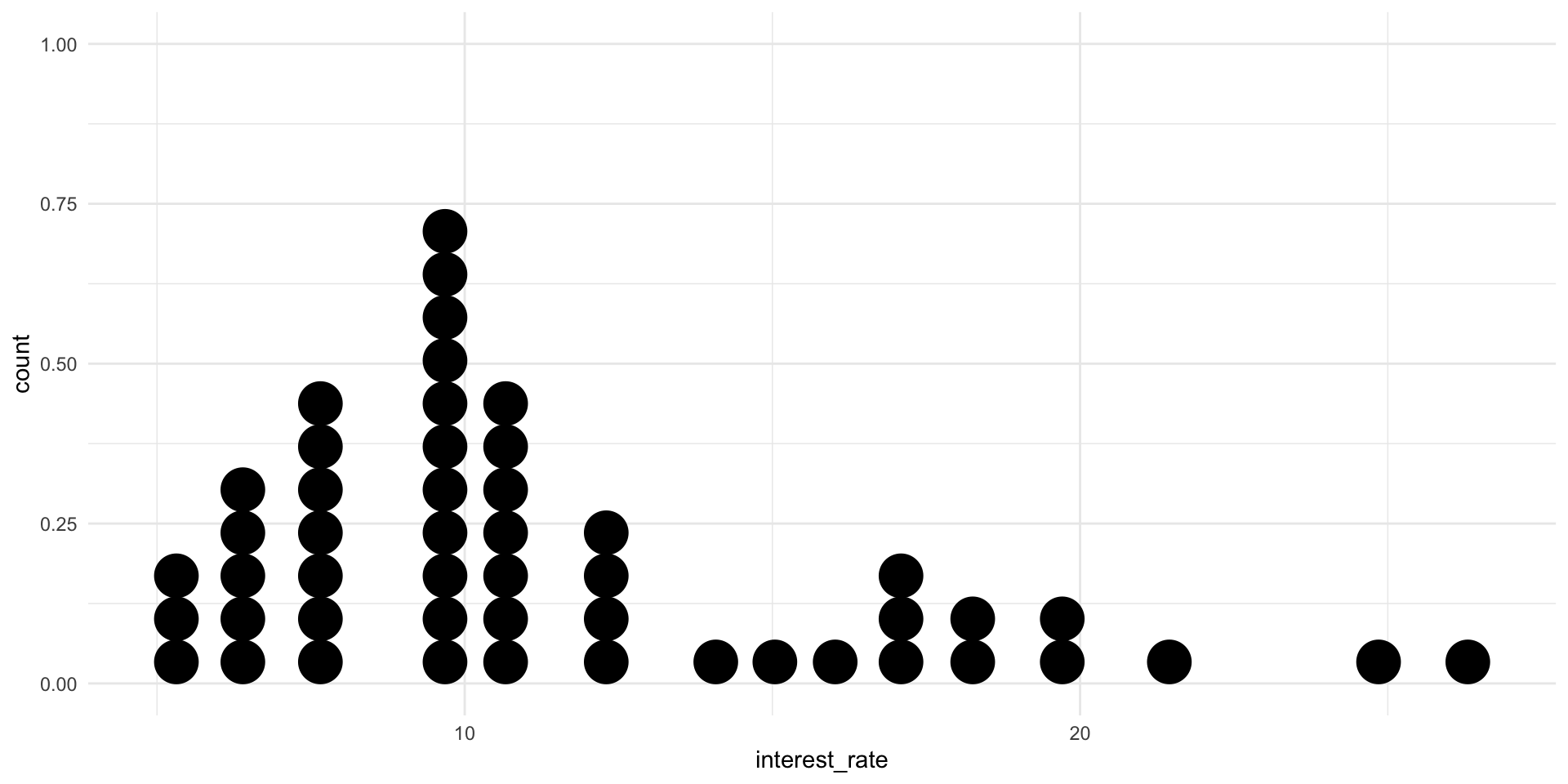
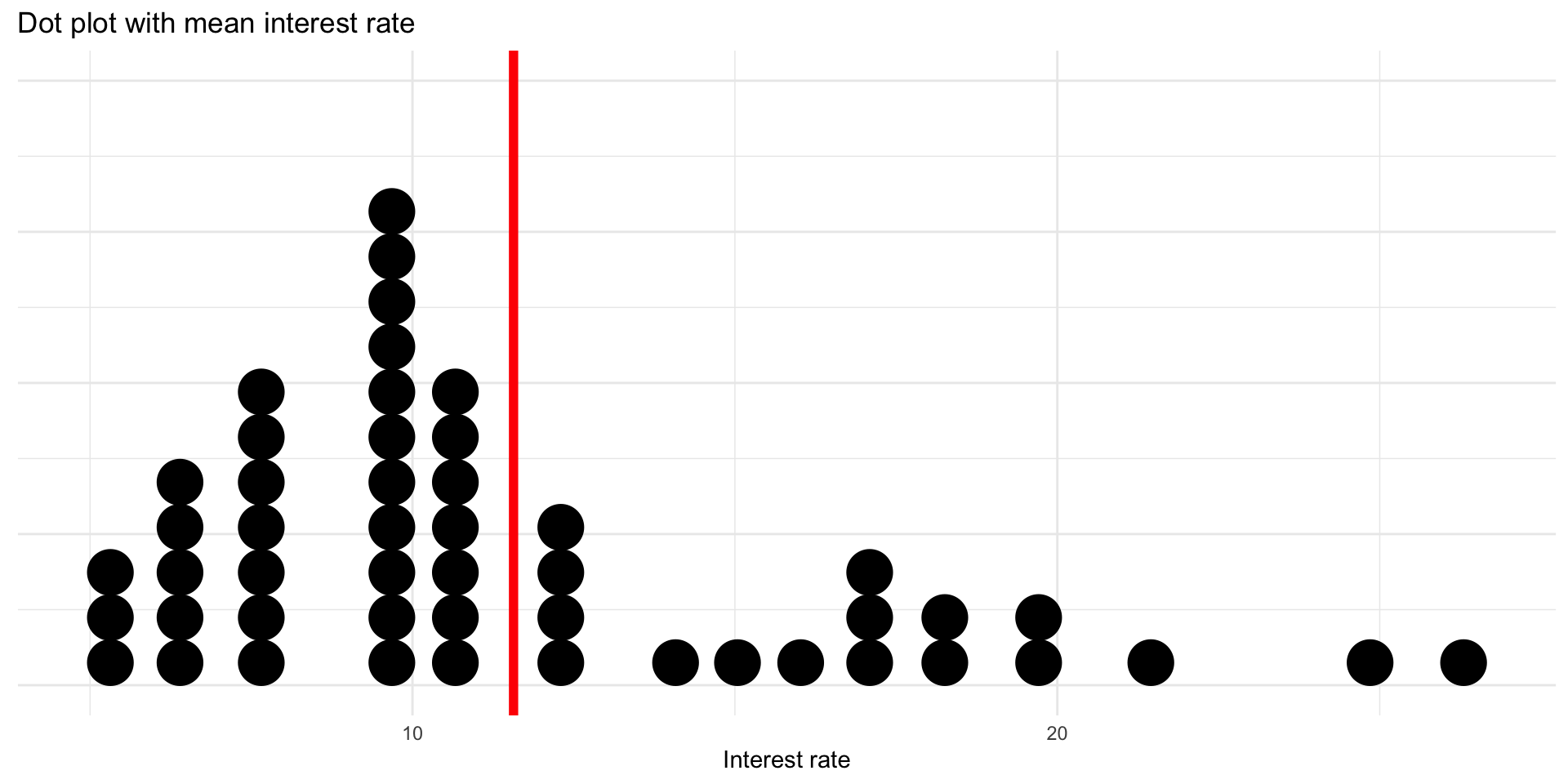
Dot plot of interest_rate

ggplot(loan50, aes(x = interest_rate)) +
  geom_dotplot()

Dot plot of with mean

• Compute mean and store in mean_interest_rate
• Add mean to plot
• Add labs

mean_interest_rate  <- loan50  |> 
  summarise(mean(interest_rate))  |> 
  pull()

ggplot(loan50, aes(x = interest_rate)) +
  geom_dotplot() +
  geom_vline(xintercept = mean_interest_rate, size = 2, color = "red") +
  labs(x = "Interest rate", y= NULL, title = "Dot plot with mean interest rate")

Your turn - dot plot

• Create a dot plot of loan_amount

• Add the median to the plot

• Add labs

• Label the loan amount on the x axis in thousands of dollars

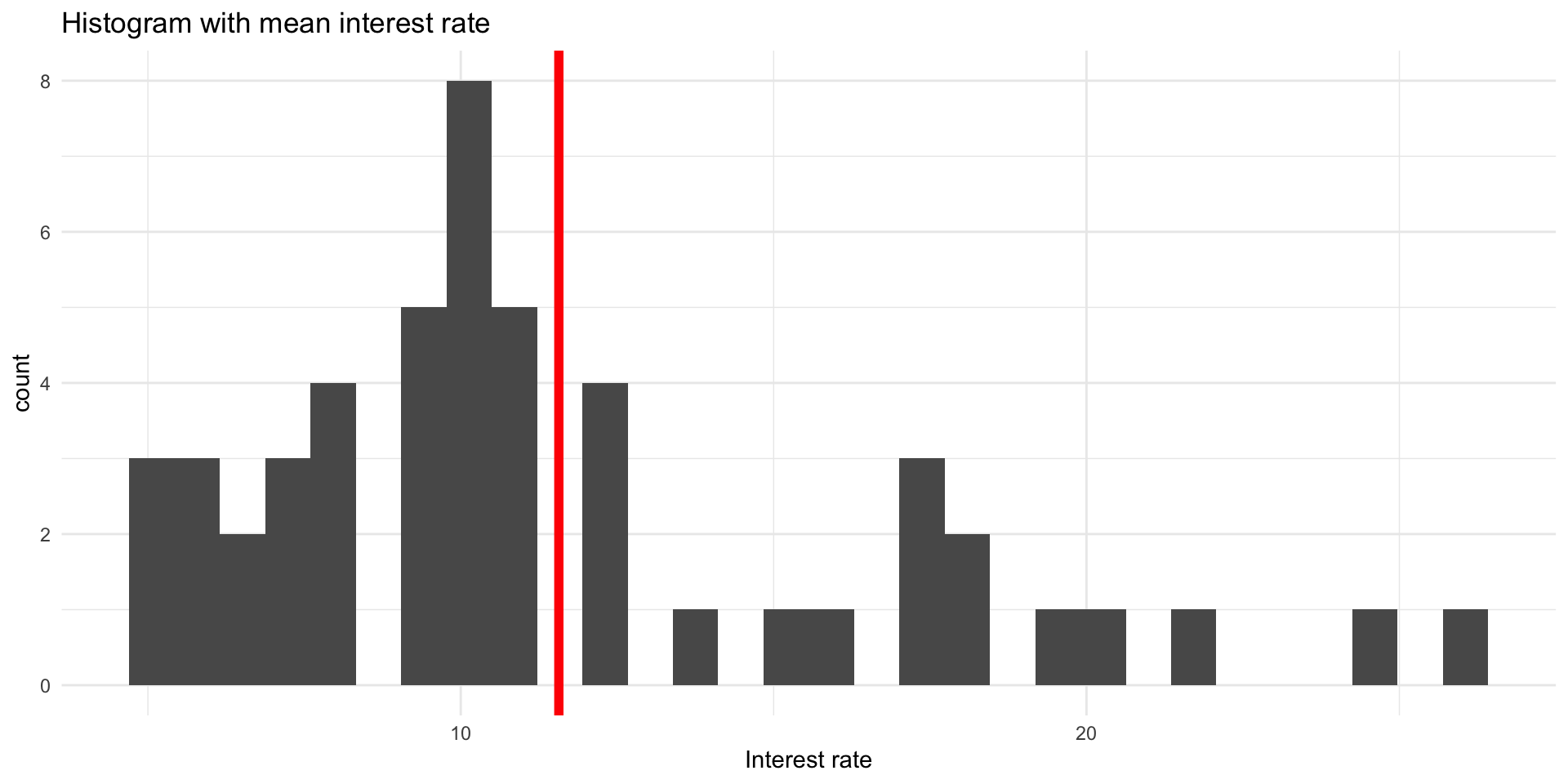
Histograms

• Dot plots show the exact value - useful for small datasets
• Histograms bins the data - useful for large datasets
• Understand shape of data distribution

ggplot(loan50, aes(x = interest_rate)) +
  geom_histogram() +
  geom_vline(xintercept = mean_interest_rate, size = 2, color = "red") +
  labs(x = "Interest rate", title = "Histogram with mean interest rate")

Shape of distribution - tails

• Longer tail left (left skewed)

• Longer tail right (right skewed)

• Equal both sides (symmetric)

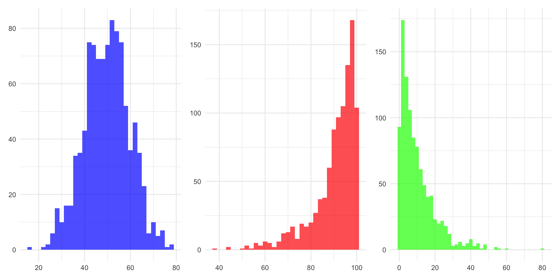
Your turn - shape

Identify which plot is symmetric, left-skewed, and right skewed.

Your turn - histogram

• Create a histogram of loan_amount

• Add the median to the plot

• Add labs

• Label the loan amount on the x axis in thousands of dollars

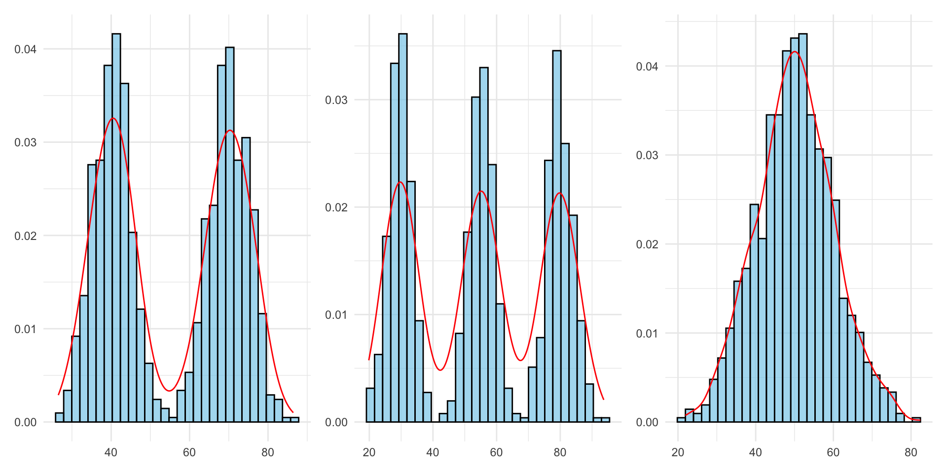
Density plot

• smoothed out histogram

ggplot(loan50, aes(x = interest_rate)) +
  geom_density() +
  geom_vline(xintercept = mean_interest_rate, size = 2, color = "red") +
  labs(x = "Interest rate", title = "Density plot with mean interest rate")

Your turn - density

• Create a density of loan_amount

• Add the median to the plot

• Add labs

• Label the loan amount on the x axis in thousands of dollars

Mode in distribution

• Prominent peak

  • unimodal

  • bimodal

  • multimodal

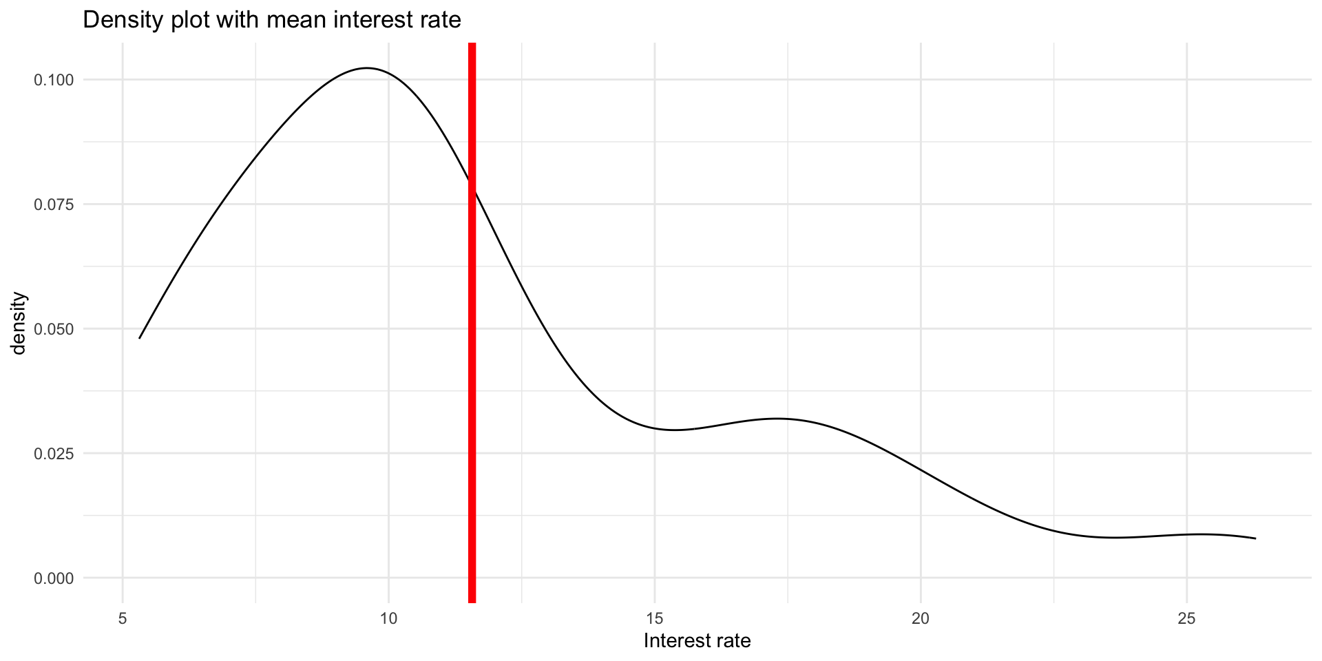
Which is unimodal, bimodal, multimodal?

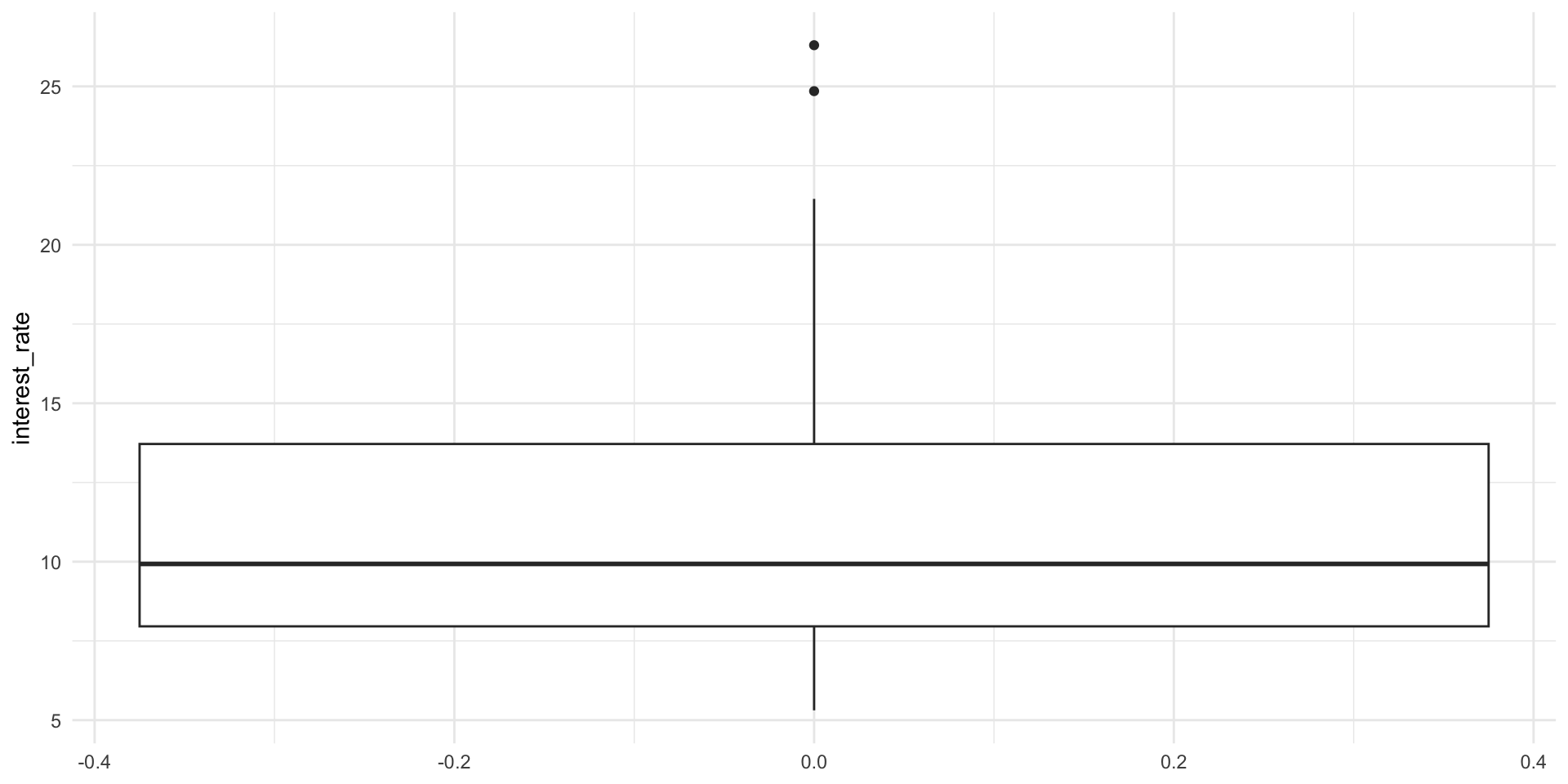
Boxplot

• similar to a histogram and density plot, a boxplot does not plot the raw data
• plots the center of the distribution (median), the values that mark off the middle half of the data (first and third quartiles), and the values that mark off the vast majority of the data (ends of the whiskers)

ggplot(loan50, aes(y = interest_rate)) +
  geom_boxplot() 

Your turn - boxplot

• Create a boxplot of loan_amount

• Add labs

• Label the loan amount on the x axis to be thousands of dollars

Summary

• types of numerical data

• plots for 1 variable

  • dot plot
  • histogram
  • density plot
  • box plot

• plots for 2 variables

  • scatterplot

Quiz

• 5 multiple choice questions using datasets in openintro package